Transportation Model: Initial Solution (Vogel’s Approximation Method), Final Solution

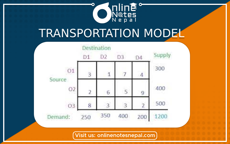
Transportation Model

The transportation model is a type of linear programming (LP) problem used to optimize the distribution of goods from several supply points (sources) to several demand points (destinations) while minimizing the total transportation costs. It is particularly useful in supply chain management, logistics, and distribution planning.

Components of the Transportation Model:

1. Suppliers (Sources): These are the points or locations from which goods are shipped. Each supplier has a fixed supply capacity.

2. Customers (Destinations): These are the points or locations where goods are delivered. Each customer has a fixed demand requirement.

3. Unit Transportation Cost (Cost Matrix): This is a matrix that represents the cost of transporting one unit of the commodity from each supplier to each customer. The rows represent the suppliers, the columns represent the customers, and the cell values indicate the transportation cost from a supplier to a customer.

4. Supply Constraints: The total supply from all suppliers cannot exceed their respective capacities.

5. Demand Constraints: The total demand from all customers must be satisfied.

Objective Function:

The objective of the transportation model is to minimize the total transportation cost, which is the sum of the product of the quantity transported from each supplier to each customer and the corresponding unit transportation cost.

Mathematical Formulation:

Let:

• S = set of suppliers (sources), i = 1, 2, ..., m
• D = set of customers (destinations), j = 1, 2, ..., n
• xᵢⱼ = quantity transported from supplier i to customer j
• cᵢⱼ = unit transportation cost from supplier i to customer j
• aᵢ = supply capacity of supplier i
• bⱼ = demand requirement of customer j

The objective function to minimize the total transportation cost is:

Minimize Z = ΣᵢΣⱼ (cᵢⱼ * xᵢⱼ)

subject to the following constraints:

1. Supply Constraints: Σⱼ xᵢⱼ ≤ aᵢ, for all i ∈ S (Total supply from supplier i)

2. Demand Constraints: Σᵢ xᵢⱼ ≥ bⱼ, for all j ∈ D (Total demand at customer j)

3. Non-Negativity Constraints: xᵢⱼ ≥ 0, for all i ∈ S, j ∈ D

Solving the Transportation Model:

The transportation model can be solved using various optimization techniques, such as the Northwest Corner Method, Least Cost Method, Vogel's Approximation Method, or specialized linear programming solvers.

1. Northwest Corner Method: It starts by allocating shipments in the top-left (northwest) corner of the cost matrix and then iteratively moves to the next unallocated cell while satisfying supply and demand constraints.

2. Least Cost Method: It selects the cell with the lowest transportation cost and allocates shipments until one of the suppliers or customers is exhausted, then moves to the next lowest cost cell.

3. Vogel's Approximation Method: This method is an improvement over the least cost method and considers the penalties for not fully utilizing the lowest cost cells.

Once the optimal allocations of shipments are determined, the total transportation cost and the quantity transported from each supplier to each customer can be obtained.

Important Notes:

1. The transportation model assumes that the total supply is equal to the total demand, i.e., Σᵢ aᵢ = Σⱼ bⱼ.

2. If the total supply is not equal to the total demand, we can introduce a "dummy" supplier or customer with zero transportation cost to balance the problem.

3. The transportation model is based on several assumptions, such as constant unit transportation costs, fixed supply and demand values, and no capacity constraints on transportation paths. In practical scenarios, these assumptions may need to be adjusted to reflect real-world complexities.

Vogel's Approximation Method (VAM):

Vogel's Approximation Method is an iterative process to find an initial feasible solution for the transportation problem. It tries to balance costs and identify the most promising allocations at each step

1. Step 1 - Calculate Penalties:

• For each row (source) and column (destination) in the transportation table, find the two smallest transportation costs.
• Calculate the difference between the two smallest costs (penalties) and enter these penalties in separate rows and columns.

2. Step 2 - Identify Maximum Penalty:

• Identify the row and column with the highest penalty.

3. Step 3 - Allocate as much as possible:

• Begin allocating units from the highest penalty cell while respecting the supply and demand constraints.
• If either the corresponding row or column is exhausted (supply/demand becomes zero), cross out the row or column and proceed to the next highest penalty.

4. Step 4 - Update Penalties:

• Recalculate the penalties for the remaining rows and columns.
• If a row or column is crossed out, ignore it while calculating penalties.

5. Step 5 - Repeat Steps 2 to 4:

• Continue the process until all supplies and demands are fully satisfied.

Final Solution:

After obtaining the initial solution using Vogel's Approximation Method, we need to check if it is feasible and optimal. The initial solution is feasible if the total supply matches the total demand, and no cell is left unallocated. To check optimality, we can use various methods like the Northwest Corner Method, Least Cost Method, or MODI (Modified Distribution) method.

If the initial solution is not optimal, we can improve it iteratively using methods like the Stepping Stone Method or UV Method. These methods involve transferring units from one allocated cell to another while maintaining supply and demand constraints until an optimal solution is reached.

To summarize, the steps to obtain the final solution are:

1. Use Vogel's Approximation Method to find an initial feasible solution.

2. Check the feasibility of the initial solution.

3. If the initial solution is not optimal, apply an improvement method (e.g., Stepping Stone Method) to iteratively improve the solution.

5. Repeat the improvement process until an optimal solution is reached, where the total transportation cost is minimized.

Once the final solution is obtained, it represents the optimal transportation plan, and the values in the cells of the transportation table indicate the quantities to be transported from sources to destinations, resulting in minimum total transportation cost.