Regression-based linear and curvilinear trend models

Regression-based linear and curvilinear trend models are used in time series analysis to capture the underlying patterns and trends in the data. These models help in understanding the relationship between the dependent variable (usually time) and the independent variable (the variable being studied). Here's a complete note on both types of trend models:

2. Linear Trend Model:

A linear trend model assumes that the relationship between the dependent variable and time is linear, which means the trend is changing at a constant rate over time. The general equation for a linear trend model is:

 

Yt​=β0​+β1​⋅t+εt​

Where:

• Yt​ represents the value of the dependent variable at time t.
• β0​ is the intercept term, which represents the value of Yt​ when t is zero.
• β1​ is the slope coefficient, which measures the change in Yt​ for each unit change in time t.
• t is the time variable.
• εt​ is the error term, representing the random variation or noise in the data.

To estimate the parameters β0​ and β1​, we use regression analysis. The least squares method is commonly employed to find the line that minimizes the sum of squared errors between the observed and predicted values.

Advantages of Linear Trend Model:

• Simple and easy to interpret.
• Suitable for data that exhibit a constant rate of change over time.

Limitations of Linear Trend Model:

• Cannot capture non-linear patterns in the data.
• Unsuitable for data with irregular fluctuations or abrupt changes in trend.

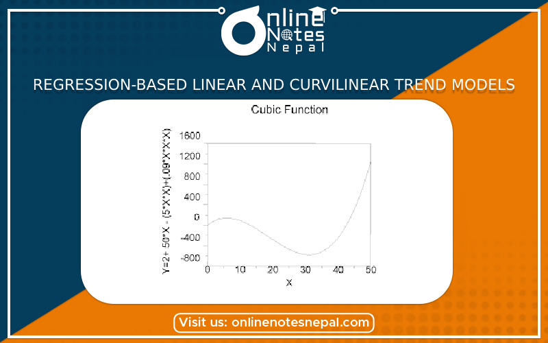
2. Curvilinear Trend Model:

A curvilinear trend model allows for non-linear relationships between the dependent variable and time. These models are more flexible than linear trend models and can capture various types of curvatures, such as quadratic, cubic, exponential, etc. The general equation for a curvilinear trend model can be represented as:

 

Yt​=β0​+β1​⋅t+β2​⋅t^2+…+βn​⋅t^n+εt​

Where:

• Yt​ represents the value of the dependent variable at time t.
• β0​,β1​,…,βn​ are the coefficients to be estimated.
• t is the time variable.
• εt​ is the error term, representing the random variation or noise in the data.

To determine the appropriate degree of curvature (n) and estimate the coefficients, various statistical techniques like polynomial regression or non-linear least squares are utilized.

Advantages of Curvilinear Trend Model:

• Can capture a wide range of non-linear patterns in the data.
• More flexible and adaptable to complex trends.

Limitations of Curvilinear Trend Model:

• Higher complexity compared to linear trend models.
• The selection of the appropriate degree of curvature can be challenging, and overfitting may occur if the degree is too high.

In summary, linear trend models assume a constant rate of change over time, while curvilinear trend models accommodate non-linear relationships. The choice between the two depends on the nature of the data and the complexity of the underlying trend. Additionally, it's essential to assess the goodness of fit and consider the predictive accuracy of the model when selecting the appropriate trend model.