Published by: Dikshya
Published date: 19 Jul 2023

Least Squares Method of Fitting Linear and Nonlinear Functions for Given Data
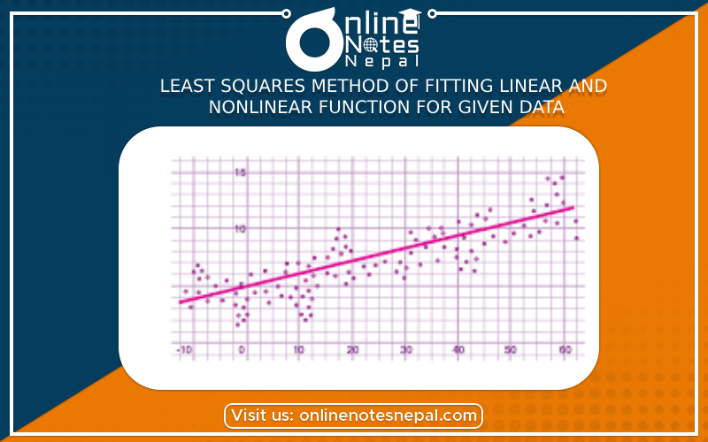
The Least Squares Method is a common technique used to find the best-fitting model for a given set of data points. It aims to minimize the sum of the squared differences (residuals) between the predicted values of the model and the actual data points. The method can be applied to both linear and nonlinear functions, although the approach and formulas differ for each case.
1. Least Squares Method for Fitting Linear Functions:
A linear function has the general form:
y = mx + b
where 'y' is the dependent variable, 'x' is the independent variable, 'm' is the slope, and 'b' is the y-intercept.
The objective is to find the values of 'm' and 'b' that minimize the sum of squared residuals, represented as S:
S = Σ(yᵢ - (mxᵢ + b))²
where (xᵢ, yᵢ) are the data points.
To find the optimal values of 'm' and 'b', we take the partial derivatives of S with respect to 'm' and 'b' and set them to zero:
∂S/∂m = 0 ∂S/∂b = 0
Solving these equations will yield the values of 'm' and 'b' that provide the best linear fit to the data.
2. Least Squares Method for Fitting Nonlinear Functions:
Nonlinear functions do not have a linear relationship between the dependent and independent variables. Examples include exponential, logarithmic, power-law, and polynomial functions.
A general form for a nonlinear function can be represented as:
y = f(x, β₁, β₂, ..., βₙ)
where 'y' is the dependent variable, 'x' is the independent variable, and β₁, β₂, ..., βₙ are the parameters of the function.
The objective is to find the optimal values of the parameters β₁, β₂, ..., βₙ that minimize the sum of squared residuals, represented as S:
S = Σ(yᵢ - f(xᵢ, β₁, β₂, ..., βₙ))²
where (xᵢ, yᵢ) are the data points.
Unlike the linear case, there is no straightforward algebraic solution to find the parameters that minimize S for nonlinear functions. Instead, iterative numerical methods like the Gauss-Newton method or the Levenberg-Marquardt algorithm are typically used.
Linear Least Squares (Fitting a straight line):
Optimal slope (m) and y-intercept (b):

where n is the number of data points.
Nonlinear Least Squares:
In the case of nonlinear functions, there is no simple closed-form solution like in the linear case. The parameters β₁, β₂, ..., βₙ need to be iteratively adjusted using numerical methods to minimize the sum of squared residuals S.
One common iterative method is the Gauss-Newton method, which approximates the nonlinear function as a linear function and iteratively updates the parameter vector:

where J is the Jacobian matrix of partial derivatives of the function f with respect to the parameters β₁, β₂, ..., βₙ, and δβ is the update vector to the parameter vector β.
This process is repeated until convergence (when the change in the parameter values becomes small).
Remember that the success of the least squares method depends on choosing an appropriate model (linear or nonlinear) that best describes the underlying relationship between the variables based on the data at hand. Additionally, be cautious about overfitting, as overly complex models can result in poor predictions for new data points.