Lagrange Interpolation

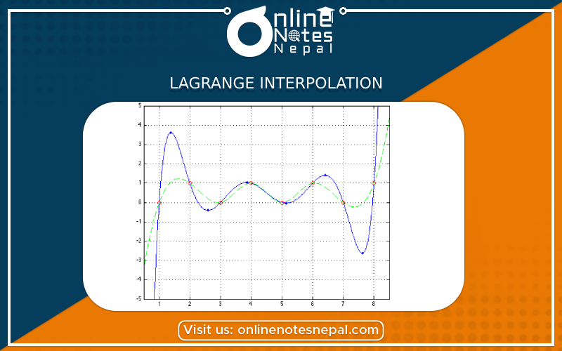
Lagrange interpolation is a mathematical method used to construct a polynomial that passes through a given set of data points. It is named after the Italian-French mathematician Joseph-Louis Lagrange. This technique is widely used in numerical analysis, numerical integration, and approximation theory. The main goal of Lagrange interpolation is to find a simple polynomial that accurately represents the given data points.

Formulation

Given a set of data points (xi, yi) for i = 0, 1, ..., n, where xi and yi are the x-coordinate and y-coordinate of the data points, respectively, the Lagrange interpolation polynomial L(x) can be expressed as:

Where:

• L(x) is the Lagrange interpolation polynomial of degree n (n is one less than the number of data points).
• xi and yi are the given data points.
• n is the number of data points in the set.

The Lagrange polynomial passes through all the given data points (xi, yi) and can be used to approximate the value of y for any x within the range of the given data points.

Advantages and Limitations

Advantages:

1. Simplicity: Lagrange interpolation provides a straightforward method to obtain an interpolating polynomial.
2. Versatility: The method can be applied to a variety of functions and data sets.
3. Accuracy: For well-behaved data sets, the Lagrange polynomial can provide accurate interpolation.

Limitations:

1. Runge's Phenomenon: The Lagrange interpolation polynomial can exhibit oscillatory behavior when interpolating over equidistant points, especially for high-degree polynomials. This issue is known as Runge's phenomenon.
2. High Degree: For a large number of data points, the degree of the Lagrange polynomial can become excessively high, leading to computational complexity and numerical instability.
3. Sensitivity: The Lagrange polynomial is sensitive to the distribution of data points, and adding or removing a data point can significantly affect the resulting polynomial.

Procedure

The Lagrange interpolation procedure involves the following steps:

1. Given a set of data points (xi, yi), calculate the Lagrange basis polynomials.

   • The Lagrange basis polynomial Li(x) for the ith data point is calculated as follows:

2. Formulate the Lagrange interpolation polynomial L(x) by combining the Lagrange basis polynomials with their corresponding y-values:

3. The resulting L(x) is the Lagrange interpolation polynomial that passes through all the given data points.

Example

Let's consider a simple example with three data points: (1, 2), (2, 4), and (3, 6).

Step 1: Calculate the Lagrange basis polynomials:

• L0(x) = ((x - 2)(x - 3)) / ((1 - 2)(1 - 3)) = (x^2 - 5x + 6) / 2
• L1(x) = ((x - 1)(x - 3)) / ((2 - 1)(2 - 3)) = -(x^2 - 4x + 3)
• L2(x) = ((x - 1)(x - 2)) / ((3 - 1)(3 - 2)) = (x^2 - 3x + 2)

Step 2: Formulate the Lagrange interpolation polynomial L(x):

• L(x) = 2 * L0(x) + 4 * L1(x) + 6 * L2(x)
• L(x) = 2 * ((x^2 - 5x + 6) / 2) + 4 * (-(x^2 - 4x + 3)) + 6 * (x^2 - 3x + 2)
• L(x) = -x^2 + 7x + 2

The Lagrange interpolation polynomial for the given data points is L(x) = -x^2 + 7x + 2.

Conclusion

Lagrange interpolation is a useful method for approximating a function or dataset using a polynomial that passes through specific points. While it has its limitations, such as Runge's phenomenon and sensitivity to data distribution, Lagrange interpolation remains a fundamental technique in numerical analysis and forms the basis for other interpolation methods.