Published by: Dikshya
Published date: 19 Jul 2023

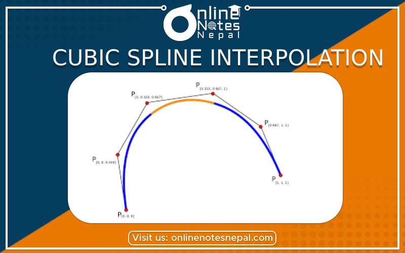
Cubic spline interpolation is a widely used technique in numerical analysis and computer graphics for approximating a smooth curve passing through a given set of data points. It is particularly useful when you want to construct a continuous and smooth curve while preserving the shape of the data points. The interpolation is achieved by dividing the data range into small intervals and fitting cubic polynomials in each interval. These polynomials, called "spline segments," are then combined to create the final spline curve.
The key characteristics of cubic spline interpolation are as follows:
Data Points: The method requires a set of data points (xᵢ, yᵢ), where 'x' represents the independent variable, and 'y' represents the dependent variable.
Interpolation Condition: Cubic spline interpolation guarantees that the resulting curve passes through all the given data points, ensuring that f(xᵢ) = yᵢ for each xᵢ in the data.
Smoothness: The spline curve is designed to be smooth across the entire range, meaning that the first and second derivatives are continuous at the data points. This smoothness provides a visually pleasing and physically realistic curve representation.
Piecewise Polynomial: Cubic spline interpolation constructs a piecewise polynomial curve, with each polynomial segment representing a small interval between two consecutive data points.
The interpolation process involves the following steps:
Step 1: Data Preprocessing Arrange the input data points in ascending order based on their 'x' values. This step ensures that the data is well-ordered, simplifying subsequent computations.
Step 2: Compute Spline Segments For each interval between data points (xᵢ, xᵢ₊₁), a cubic polynomial is computed to interpolate the data in that interval. This polynomial is typically represented in the form:
Sᵢ(x) = aᵢ + bᵢ(x - xᵢ) + cᵢ(x - xᵢ)² + dᵢ(x - xᵢ)³
where 'aᵢ', 'bᵢ', 'cᵢ', and 'dᵢ' are coefficients determined based on interpolation conditions and smoothness requirements.
Step 3: Derive Coefficients To determine the coefficients 'aᵢ', 'bᵢ', 'cᵢ', and 'dᵢ', the method uses the following set of equations:
aᵢ = yᵢ bᵢ = (yᵢ₊₁ - yᵢ) / (xᵢ₊₁ - xᵢ) cᵢ = hᵢyᵢ₊₁ - hᵢ₊₁yᵢ / 6 dᵢ = (hᵢ₊₁yᵢ - hᵢyᵢ₊₁) / 6hᵢ
where 'hᵢ = xᵢ₊₁ - xᵢ' represents the interval width between data points.
Step 4: Construct the Spline Curve Combine all the individual spline segments (Sᵢ(x)) into a single continuous curve that passes through each data point. This resulting spline curve represents the cubic spline interpolation.
Advantages of Cubic Spline Interpolation:
Accuracy: Cubic splines provide higher accuracy than linear interpolation methods because of their ability to capture more complex curves.
Smoothness: The resulting spline curve is smooth and continuous, which is essential in many applications like computer graphics and animation.
Data Preservation: Unlike some other interpolation techniques, cubic splines ensure that the interpolating curve passes through all the original data points, preserving their values.
Low Oscillation: Cubic splines tend to have lower oscillation between data points, making them suitable for generating smooth trajectories.
In conclusion, cubic spline interpolation is a powerful method for generating smooth and accurate curves that pass through a given set of data points. Its widespread applications include computer graphics, animation, data visualization, and engineering simulations, where the preservation of data integrity and curve smoothness are crucial.