Process Scheduling algorithms

Different time with respect to a process

• Arrival Time(AT): Time at which the process arrives in the ready queue.
• Burst Time (BT): Time required by a process for CPU execution.
• Completion Time(CT): Time at which the process completes its execution.
• Turn Around Time(TAT): The time interval from the time of submission of a process to the time of the completion of the process.
  OR,
  Time Difference between completion time and arrival time. i.e. TAT= CT - AT
• Waiting Time(WT): The total time waiting in a ready queue.
  OR,
  Time Difference between turnaround time and burst time. i.e.WT = TAT - BT
• Response time(RT): Amount of time from when a request was submitted until the first response is produced.
• Quantum size: It is the specific time interval used to prevent anyone process from monopolizing the system i.e. can be run exclusively.

A Process Scheduler schedules different processes to be assigned to the CPU based on particular scheduling algorithms. The rule or set of rules that are followed to schedule the process is known as the process scheduling algorithm. The algorithms are either non-preemptive or preemptive.

Some of the algorithms are:

1.  First Come First Serve (FCFS) Scheduling

• It is a non-preemptive scheduling algorithm.
• The process which arrives first gets executed first or the process which requests the CPU first, gets the CPU allocated first
• First Come First Serve, is just like FIFO (First in First out) Queue data structure, where the data element which is added to the queue first, is the one who leaves the queue first.
• A perfect real-life example of FCFS scheduling is buying tickets at the ticket counters.

Advantages

•  FCFS algorithm doesn't include any complex logic, it just puts the process requests in a queue and executes them one by one. Hence, FCFS is pretty simple and easy to implement.
• Eventually, every process will get a chance to run, so starvation doesn't occur.

Disadvantages

• There is no option for preemption of a process. If a process is started, then the CPU executes the process until it ends.
• Because there is no preemption, if a process executes for a long time, the processes in the back of the queue will have to wait for a long time before they get a chance to be executed.

Example 1: Consider the following set of processes having their arrival time and CPU-burst time. Find the average waiting time and turnaround time using FCFS.

Process	Arrival Time (ms)	Burst Time (ms)
P1	0	4
P2	1	3
P3	2	1
P4	3	2
P5	4	5

Solution:
Preparing Gantt chart using FCFS we get,

We know,
TAT (Turnaround Time) = CT (Completion Time) – AT (Arrival Time) and
WT (Waiting Time) = TAT (Turnaround Time) – BT (Burst Time)
Now finding TAT and WT,

Process	AT	BT	CT	TAT	WT
P1	0	4	4	4	0
P2	1	3	7	6	3
P3	2	1	8	6	5
P4	3	2	10	7	5
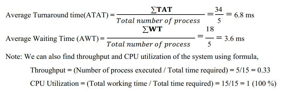
P5	4	5	15	11	6
				∑TAT= 34	∑WT= 18

 

Example 2: Consider the given processes with arrival and burst time given below. Schedule the given processes using FCFS and find average waiting time and average turn-around time.

PROCESSES	ARRIVAL TIME	BURST TIME
A	0	3
B	2	6
C	4	4
D	6	5
E	8	2
F	3	4

SOLUTION:
Applying FCFS Gantt chart for the given processes becomes:

Now, from the Gantt chart,

Process	Arrival time (AT)	Burst time (BT)	Completion time (CT)	Turnaround time TAT = CT – AT	Waiting time WT=TAT-BT
A	0	3	3	3	0
B	2	6	9	7	1
C	4	4	17	13	9
D	6	5	22	16	11
E	8	2	24	16	14
F	3	4	13	10	6
				∑ TAT=65	∑ WT=41

Average turn-around time = ∑(TAT) / n = 65/6 = 10.83
Average waiting time = ∑(WT) / n =41/6 = 6.83

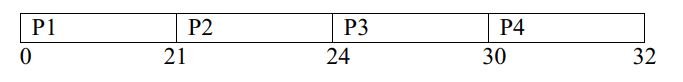
Example 3: Consider the processes P1, P2, P3, P4 given in the below table, arrives for execution in the same order, with Arrival Time 0, and given Burst Time, find the average waiting time using the FCFS scheduling algorithm.

Process	Burst Time (ms)
P1	21
P2	3
P3	6
P4	2

Solution:

Now from the Gantt chart,

Process	Arrival Time (ms)	Burst Time	Completion Time	Turnaround Time TAT=CT-AT	Waiting Time WT = TAT - BT
P1	0	21	21	21	0
P2	0	3	24	24	21
P3	0	6	30	30	24
P4	0	2	32	32	30

Average WT = (0+21+24+30)/4 = 18.75

2. Shortest Job First (SJF) Scheduling

• It is a non-preemptive scheduling algorithm.
• It is also known as shortest job next (SJN)
• It is a scheduling policy that selects the waiting process with the smallest execution time
  to execute next.

Advantages:

• The throughput is increased because more processes can be executed in less amount of time.
• Having minimum average waiting time among all scheduling algorithms.

Disadvantages:

• It is practically infeasible as Operating System may not know burst times and therefore may not sort them.
• Longer processes will have more waiting time, eventually, they'll suffer starvation.

Example 1: Consider the given processes with arrival and burst time given below. Schedule the given processes using SJF and find average waiting time (AWT) and average turnaround time(ATAT).

PROCESSES	ARRIVAL TIME	BURST TIME
A	0	7
B	2	5
C	3	1
D	4	2
E	5	3

Solution:
According to the given question, the Gantt chart for SJF given processes becomes:

Now,
Calculating of TAT and WT using: TAT= CT – AT and WT = TAT - BT

Process	Arrival time	Burst time	Completion time	Turn-around time	Waiting time
A	0	7	7	7	0
B	2	5	18	16	11
C	3	1	8	5	4
D	4	2	10	6	4
E	5	3	13	8	5
				∑TAT=42	∑WT=24

Average turn-around time = ∑(TAT) / n = 42/5 = 10.83
Average waiting time = ∑(WT) / n =24/5 = 4.8

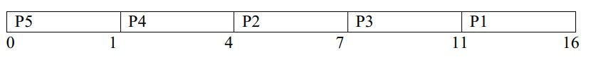
Example 2: Five processes P1, P2, P3, P4, and P5 having burst time 5,3,4,3,1 arrives at CPU. Find the Average TAT and Average WT using the Shortest job first scheduling algorithm.

PROCESSES	BURST TIME (ms)
P1	5
P2	3
P3	4
P4	3
P5	1

Solution
Since there is no arrival time so it is assumed all the processes arrive initially. i.e. AT=0
The Gantt chart for the above processes becomes:

Now, using the Gantt chart above and formula,

TAT = (CT-AT) and WT = (TAT-BT)

Process	Arrival time	Burst time	CT	TAT	WT
P1	0	5	16	16	11
P2	0	3	7	7	4
P3	0	4	11	11	7
P4	0	3	4	4	1
P5	0	1	1	1	0
				∑TAT=39	∑WT=23

Average turn-around time = ∑(TAT) / n = 39/5 = 7.8 ms
Average waiting time = ∑(WT) / n =23/5 = 4.6 ms

Example 3: Consider the given processes with arrival and burst time given below. Schedule the given processes using SJF and find waiting time and turn-around time.

PROCESSES	ARRIVAL TIME	BURST TIME
A	1	7
B	2	5
C	3	1
D	4	2
E	5	8

Solution
The Gantt chart for the above processes becomes:
Here no process arrives at time= 0, so the CPU stays in an idle position.

Now, using the Gantt chart above and formula,
TAT = (CT-AT) and WT = (TAT-BT)

Process	Arrival time	Burst time	CT	TAT	WT
A	1	7	8	7	0
B	2	5	16	14	9
C	3	1	9	6	5
D	4	2	11	7	5
E	5	8	24	19	11

Here Throughput = (5/24) and CPU Utilization = (23/24) of time.   since CPU stay in idle for 1 unit of time.

3. Shortest Remaining Time (SRT) Scheduling

• It is a preemptive scheduling algorithm.
• It is also called Preemptive shortest job first or Shortest remaining time next or Shortest remaining time first.
• In this scheduling algorithm, the process with the smallest amount of time remaining until completion is selected to execute. Since the currently executing process is the one with the shortest amount of time remaining by definition, and since that time should only reduce as execution progresses, processes will always run until they complete or a new process is added that requires a smaller amount of time.

Advantage:

• Short processes are handled very quickly.
• The system also requires very little overhead since it only makes a decision when a process completes or a new process is added.
• When a new process is added the algorithm only needs to compare the currently executing process with the new process, ignoring all other processes currently waiting to execute.

Disadvantage:

• Like shortest job first, it has the potential for process starvation.
• Long processes may be held off indefinitely if short processes are continually added.

Example 1: Consider the following processes with arrival time and burst time. Schedule them using SRT.

PROCESSES	ARRIVAL TIME(AT)	BRUST TIME (BT)
A	0	7
B	1	5
C	2	3
D	3	1
E	4	2
F	5	1

Solution:
Gantt chart for the above processes becomes:

 

Process	Arrival time	Burst time	CT	TAT	WT
A	0	3	19	19	12
B	2	6	13	12	7
C	4	5	6	4	1
D	6	4	4	1	0
E	8	2	9	5	3
F	5	1	7	2	1
				∑TAT=43	∑WT=24

Average turn-around time = ∑(TAT) / n = 43/6 = 7.16 units
Average waiting time = ∑(WT) / n =24/6 = 4 units

4.  Priority Scheduling

•  In this scheduling, Priority is assigned for each process.
•  The process with the highest priority is executed first and so on.
• Processes with the same priority are executed in an FCFS manner.
• Priority can be decided based on memory requirements, time requirements, or any other resource requirement

Advantages of Priority Scheduling:

• The priority of a process can be selected based on memory requirement, time requirement, or user preference. For example, a high-end game will have better graphics, which means the process which updates the screen in a game will have higher priority so as to achieve better graphics performance.

Disadvantages:

• A second scheduling algorithm is required to schedule the processes which have the same priority.
• In preemptive priority scheduling, a higher priority process can execute ahead of an already executing lower priority process. If the lower priority process keeps waiting for higher-priority processes, starvation occurs.

Priority scheduling is of both types: preemptive and non-preemptive.

a. Non-Preemptive Priority Scheduling

• In the Non Preemptive Priority scheduling, The Processes are scheduled according to the priority number assigned to them.
• Once the process gets scheduled, it will run till the completion.
• Generally, the lower the priority number, the higher is the priority of the process.

Example 1: There are 7 processes P1, P2, P3, P4, P5, P6, and P7. Their priorities, Arrival Time and burst time are given at the table. Find waiting time and response time using non-preemptive priority scheduling. Also, find the average WT.

Process	Priority	Arrival Time	Burst Time
P1	2	0	3
P2	6	2	5
P3	3	1	4
P4	5	4	2
P5	7	6	9
P6	4	5	4
P7	10	7	10

Solution:
Gantt chart for the process is:

From the GANTT Chart prepared, we can determine the completion time of every process. The turnaround time, waiting time, and response time will be determined.
Turn Around Time = Completion Time - Arrival Time
Waiting Time = Turn Around Time - Burst Time
Response time = Time at which process get a first response – Arrival Time

Process	Priority	Arrival Time	Burst Time	Completion Time	Turnaround Time	Waiting Time	Response Time
P1	2	0	3	3	3	0	0
P2	6	2	5	18	16	11	13
P3	3	1	4	7	6	2	3
P4	5	4	2	13	9	7	11
P5	7	6	9	27	21	12	18
P6	4	5	4	11	6	2	7
P7	10	7	10	37	30	18	27

Average Waiting Time = (0+11+2+7+12+2+18)/7 = 52/7 units

Example 2: Consider the given processes below. Schedule the algorithm using non-preemptive priority, schedule the given processes. Assume 12 is the highest priority and 2 is the lowest priority.

Process	AT	BT (ms)	PRIORITY
A	0	4	2(lowest)
B	1	2	4
C	2	3	6
D	3	5	10
E	4	1	3
F	5	4	12(highest)
G	6	6	9

Solution:

b. Preemptive Priority Scheduling

In Preemptive Priority Scheduling, at the time of arrival of a process in the ready queue, its priority is compared with the priority of the other processes present in the ready queue as well as with the one which is being executed by the CPU at that point of time. The One with the highest priority among all the available processes will be given the CPU next.

Example 1: Consider the given processes below. Schedule the algorithm using the preemptive priority algorithm and hence find AWT and ATAT. Assume 12 is the highest priority and 2 as the lowest priority.

Process	AT	BT (ms)	PRIORITY
A	0	4	2(lowest)
B	1	2	4
C	2	3	6
D	3	5	10
E	4	1	3
F	5	4	12(highest)
G	6	6	9

Solution:
The Gantt chart for the given processes becomes: -

Now,

Process	AT	BT	PRIORITY	CT	TAT	WT
A	0	4	2	25	25	21
B	1	2	4	21	20	18
C	2	3	6	20	18	15
D	3	5	10	12	9	4
E	4	1	3	22	18	17
F	5	4	12	9	4	0
G	6	6	9	18	12	6
					∑TAT=106	∑WT=81

Average turn-around time= (∑TAT=106)/7 = 15.14 ms
Average waiting time will be = (∑WT=81)/7 =11.57 ms

5. Round Robin Scheduling

• CPU is assigned to the process for a fixed amount of time.
• This fixed amount of time is called a time quantum or time slice.
• After the time quantum expires, the running process is preempted and sent to the ready queue.
• Then, the processor is assigned to the next arrived process.
• It is always a preemptive scheduling algorithm

Advantages:

• It gives the best performance in terms of average response time.
• It is best suited for the time-sharing systems, client-server architecture, and interactive systems.

Disadvantages:

• It leads to starvation for processes with larger burst times as they have to repeat the cycle many times.
• Its performance heavily depends on time quantum.
• Priorities cannot be set for the processes.

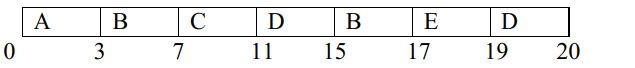
Example 1: Consider the following processes with AT and BT given. Find waiting time and turnaround time using round robin with time quantum = 4.

PROCESSES	ARRIVAL TIME(AT)	BURST TIME (BT)
A	0	3
B	2	6
C	4	4
D	6	5
E	8	2

Solution:
Ready Queue: ABCDBED
Gantt chart:

Now,

Process	Arrival time	Burst time	CT	TAT	WT
A	0	3	3	3	0
B	2	6	17	15	9
C	4	5	11	7	2
D	6	4	20	14	10
E	8	2	19	11	9

vi. HRRN (Highest Response Ratio Next)

• Highest Response Ratio Next (HRNN) is one of the most optimal scheduling algorithms.
• This is a non-preemptive algorithm in which, the scheduling is done on the basis of an extra parameter called Response Ratio.
• A Response Ratio is calculated for each of the available jobs and the Job with the highest response ratio is given priority over the others.
  Response Ratio is calculated by the given formula,
  Response Ratio = (WT+BT)/BT
  Where,
  WT → Waiting Time
  BT → Service Time or Burst Time

Advantages-

• It performs better than SJF Scheduling.
• It not only favors the shorter jobs but also limits the waiting time for longer jobs.

Disadvantages-

• It cannot be implemented practically. This is because the burst time of the processes cannot be known in advance.

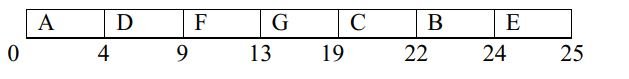
Example: Consider the following processes with AT and BT given. Find waiting time and turnaround time using HRRN.

PROCESSES	ARRIVAL TIME(AT)	BURST TIME (BT)
A	0	3
B	2	6
C	4	4
D	6	5
E	8	2

Solution:

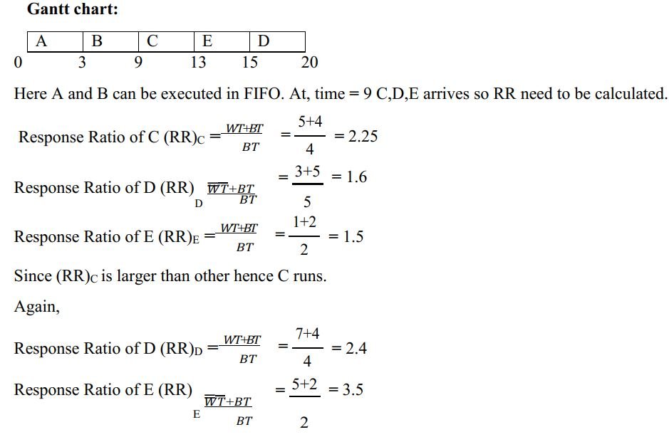
Since (RR)E is larger than others hence E runs.
Now from the Gantt chart:

Process	Arrival time (AT)	Burst time (BT)	Completion time (CT)	Turnaround time TAT = CT – AT	Waiting time WT=TAT-BT
A	0	3	3	3	0
B	2	6	9	7	1
C	4	4	13	9	5
D	6	5	20	14	9
E	8	2	15	7	5

 

 

7.  Real-Time Scheduling

• A real-time system is one in which time plays an essential role since processing should be done within the defined time limit otherwise the system will fail.
• Generally, in this type of system, one or more physical devices external to the computer generates the real-time data (stimuli) and the computer must react appropriately to them within a fixed amount of time.
• The algorithm that is used to schedule such a real-time system periodically is known as Real-Time Scheduling Algorithm.
• E.g. the computer attached with Compact Disc Player gets the bits as they come from the drive and must start converting them into music with a very tight time interval.
• If the calculation takes too long the music sounds peculiar.
• Other example includes Autopilot aircraft, Robot control in automated factory, Patient monitoring factory(ICU), etc.

Real-Time scheduling algorithm includes:

i. Rate Monotonic Algorithm (RM)
This is a fixed priority algorithm and follows the philosophy that higher priority is given to tasks with higher frequencies. Likewise, the lower priority is assigned to tasks with lower frequencies. The scheduler at any time always chooses the highest priority task for execution. By approximating to a reliable degree the execution times and the time that it takes for system handling functions, the behavior of the system can be determined a priority.

ii. Earliest Deadline First Algorithm(EDF)
This algorithm takes the approach that tasks with the closest deadlines should be meted out the highest priorities. Likewise, the task with the latest deadline has the lowest priority. Due to this approach, the processor idle time is zero and so 100% utilization can be achieved.

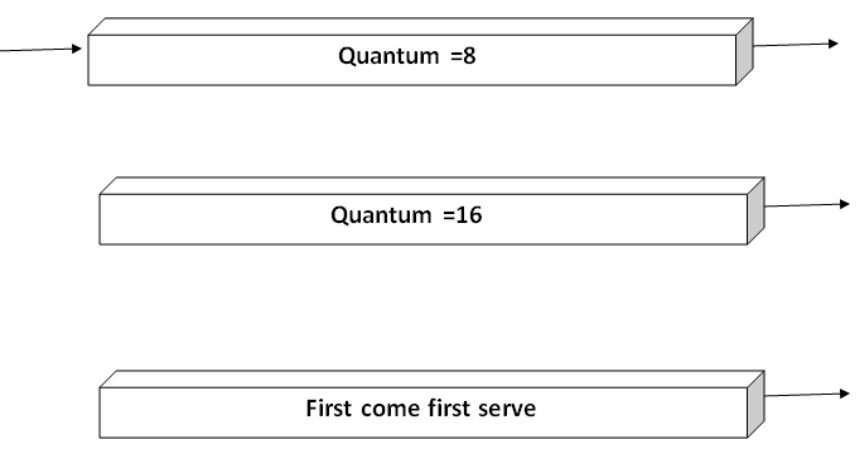
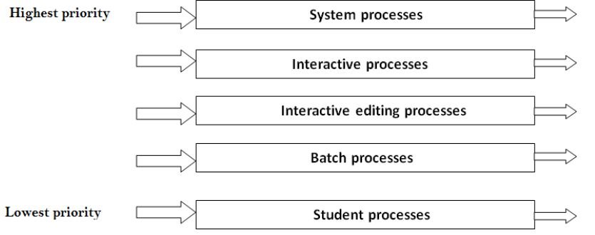
8. Multilevel Queue

• In the multilevel queue scheduling algorithm partition the ready queue has divided into seven separate queues. Based on some priority of the process; like memory size, process priority, or process type these processes are permanently assigned to one queue.
• Each queue has its own scheduling algorithm. For example, some queues are used for the foreground process and some for the background process.
• The foreground queue can be scheduled by using a round-robin algorithm while the background queue is scheduled by a first come first serve algorithm.
• It is said that there will be scheduled between the queues which are easily implemented as a fixed-priority preemptive scheduling.

Let us take an example of a multilevel queue scheduling algorithm with five queues:

• System process
•  Interactive processes
• Interactive editing processes
• Batch processes
• Student processes

9. Multilevel Feedback Queue

• In a multilevel queue scheduling, algorithm processes are permanently stored in one queue in the system and do not move between the queue.
• There is some separate queue for foreground or background processes but the processes do not move from one queue to another queue and these processes do not change their foreground or background nature, this type of arrangement has the advantage of low
  scheduling but it is inflexible in nature.
• Multilevel feedback queue scheduling allows a process to move between the queue. This the process are separate with different CPU burst time.
• If a process uses too much CPU time, then it will be moved to the lowest priority queue.
• This idea leaves I/O bound and interactive processes in the higher priority queue.
• Similarly, the process which waits too long in a lower priority queue may be moved to a higher priority queue. This form of aging prevents starvation.

The multilevel feedback queue scheduler has the following parameters:

• The number of queues in the system.
• The scheduling algorithm for each queue in the system.
• The method used to determine when the process is upgraded to a higher-priority queue.
• The method used to determine when to demote a queue to a lower-priority queue.
•  The method used to determine which process will enter in the queue and when that process needs service.